MetaTiME for Cell State Annotator and Cell Signature Mapper

installation for colab

[4]:

##Calling matplotlib first help avoid error in colab when plotting
import matplotlib
import matplotlib.pyplot as plt
!wget -q https://www.dropbox.com/s/gnmgfxa85basvwq/logo.png
img = matplotlib.image.imread('./logo.png', 0)

logo = plt.imshow( img ) # for test the colab matplotlib. a logo shall be plotted:)
_=plt.axis('off')

## install
!pip install scanpy
!pip install metatime
!pip install anndata
!pip install adjustText
!pip install leidenalg
!pip install harmonypy

imports

[1]:

import sys
import os
import numpy as np
import pandas as pd
import matplotlib.pyplot as plt
plt.rcParams['figure.dpi'] = 200
import seaborn as sns
import scanpy as sc


import importlib as imp
import metatime
import matplotlib
import matplotlib.pyplot as plt
"""
## For local testing in dev
METATIME_DIR = '../../metatime/'
if METATIME_DIR not in sys.path:
    sys.path.append(METATIME_DIR)
file = '../notebooks_dev/BCC_GSE123813_aPD1_with_metainfo.h5ad'
##
"""

from metatime import config
from metatime import loaddata
from metatime import mecmapper
from metatime import mecs
from metatime import annotator
from metatime import plmapper
from metatime import dmec
import matplotlib

Get sample data

[ ]:

#!wget -O testdata.h5ad https://www.dropbox.com/s/0sj6gtppsfr2ouo/NSCLC_GSE117570_res.pp.h5ad?dl=0

!wget -O testdata.h5ad https://www.dropbox.com/s/f791mv3tnhs9fii/BCC_GSE123813_aPD1_with_metainfo.h5ad

Load scRNA data

[ ]:

file = 'testdata.h5ad'

Or provide path to local file

[3]:

# file = '../notebooks_dev/BCC_GSE123813_aPD1_with_metainfo.h5ad' # Yost et al. 2019 Nat Med.

Load data

[3]:

adata = loaddata.load(file = file)

 Loaded ../notebooks_dev/BCC_GSE123813_aPD1_with_metainfo.h5ad

Processing and Harmonize

If your data contains count matrix, we provide a wrapped function for pre-processing the data.

Otherwise, if the data is already depth-normalized, log-transformed, and cells are filtered, we can skip this step.

[21]:

# adata = loaddata.adatapp( adata )

The sample data has multiple patients , and we can use batch correction on patients.

[4]:

batchcols = ['patient']
adata = loaddata.batchharmonize( adata, batchcols = batchcols, random_state = 0 )

[Log ] hamonize with batch  ['patient']

2023-03-14 11:18:26,769 - harmonypy - INFO - Iteration 1 of 10
2023-03-14 11:19:26,441 - harmonypy - INFO - Iteration 2 of 10
2023-03-14 11:20:26,466 - harmonypy - INFO - Iteration 3 of 10
2023-03-14 11:21:32,953 - harmonypy - INFO - Iteration 4 of 10
2023-03-14 11:22:26,570 - harmonypy - INFO - Iteration 5 of 10
2023-03-14 11:23:18,462 - harmonypy - INFO - Iteration 6 of 10
2023-03-14 11:24:01,069 - harmonypy - INFO - Iteration 7 of 10
2023-03-14 11:24:29,524 - harmonypy - INFO - Iteration 8 of 10
2023-03-14 11:25:14,176 - harmonypy - INFO - Iteration 9 of 10
2023-03-14 11:26:07,662 - harmonypy - INFO - Iteration 10 of 10
2023-03-14 11:26:58,323 - harmonypy - INFO - Stopped before convergence

[Log ] Recomputing umap

It is recommended that malignant cells are identified first and removed for best practice in cell state annotation.

In the BCC data, the cluster of malignant cells are identified with inferCNV. We can use the pre-saved column ‘isTME’ to keep Tumor Microenvironment cells

[5]:

adata = adata[adata.obs['isTME']]

We can over-cluster the cells which is useful for fine-grained cell state annotation.

[6]:

adata = annotator.overcluster( adata ) # this generates a 'overcluster' columns in adata.obs

/homes6/yiz/Tools/pip/pippy3/lib/python3.7/site-packages/scanpy/tools/_leiden.py:160: ImplicitModificationWarning: Trying to modify attribute `.obs` of view, initializing view as actual.
  categories=natsorted(map(str, np.unique(groups))),

Load MetaTiME trained model for TME

Next, let’s load the pre-computed MetaTiME MetaComponents (MeCs), and their functional annotation.

[7]:

# Load the pre-trained MeCs
mecmodel = mecs.MetatimeMecs.load_mec_precomputed()

# Load functional annotation for MetaTiME-TME
mectable = mecs.load_mecname( mecDIR = config.SCMECDIR, mode ='table' )
mecnamedict = mecs.getmecnamedict_ct(mectable)

Project on MeC space

We can project each cell onto this functional MeC space.

[8]:

pdata = mecmapper.projectMecAnn(adata, mecmodel.mec_score)

/liulab/yiz/proj/MetaTiME/metatime/mecmapper.py:151: FutureWarning: X.dtype being converted to np.float32 from float64. In the next version of anndata (0.9) conversion will not be automatic. Pass dtype explicitly to avoid this warning. Pass `AnnData(X, dtype=X.dtype, ...)` to get the future behavour.
  adataproj = anndata.AnnData( projected, obs = adata.obs )

Per-cell score projected on MeC space

Convert to table to look at per-cell projection scores

[9]:

projmat, mecscores = annotator.pdataToTable(pdata, mectable, gcol = 'overcluster')
mecscores

[9]:

	0: Pan_Interferon-response	1: Pan_Proliferation-S	2: Pan_Heat-stress	3: DC_pDC	4: B_Plasma	5: Pan_Proliferation-G2-M	6: DC_cDC2-MHCII	7: T_Treg-T-co-signaling	8: T_NK-cytotoxic	9: M_Monocyte-CD16	...	77: B_Plasma-JCHAIN	78: T_CD4T-IL7R	MeC_79	MeC_80	81: Stroma_Fibroblast-VEGF	MeC_82	83: Pan_Myeloid-fibroblast	MeC_84	MeC_85	overcluster
bcc.su001.pre.tcell_AAACCTGCAGGGATTG	-0.819890	-0.688164	-1.293394	-0.623175	-0.619621	-0.014213	-0.421470	-0.575049	0.806688	-0.228148	...	-0.503919	1.365941	0.532829	1.303657	-0.015501	-0.200811	2.227211	-2.101272	0.964769	103
bcc.su001.pre.tcell_AAACGGGCATAGACTC	0.497730	-0.781702	-1.236870	-0.225077	-0.407063	-0.196667	-0.708806	0.148677	1.226127	0.229111	...	-0.964028	-0.869057	-0.948729	0.932158	-1.617307	-0.813145	-0.541694	-1.985215	0.821645	71
bcc.su001.pre.tcell_AAACGGGTCATACGGT	-0.853597	0.389129	2.834898	-0.235956	0.469343	0.946867	-0.673814	0.078563	1.469857	0.388126	...	-0.713808	1.094122	1.178537	-2.930747	-2.534621	1.399297	-0.640663	2.175453	-1.674753	9
bcc.su001.pre.tcell_AAAGATGAGACAGGCT	1.643644	-0.217423	-0.643116	0.088754	-0.523546	-1.255705	-0.849190	0.658166	-0.770305	1.756781	...	-1.132153	1.547834	-1.547482	0.496351	-1.177201	-0.764956	0.551764	0.479404	-0.165305	8
bcc.su001.pre.tcell_AAAGATGTCTGAGTGT	-0.904096	-0.855004	-1.025405	-0.417323	-0.265433	-0.517993	-0.371883	-0.238967	-1.225588	0.211766	...	0.743283	2.142204	0.523307	0.401327	-0.243886	-0.139409	1.541129	-0.646087	-0.965725	40
...	...	...	...	...	...	...	...	...	...	...	...	...	...	...	...	...	...	...	...	...	...
bcc.su012.post.tcell_TTTGCGCGTCTTTCAT	-0.655006	-0.323290	1.357172	-0.252120	-0.477362	-0.562883	-0.469015	-0.594926	-0.978787	0.131918	...	0.224142	1.476642	1.258007	-0.838055	0.543334	0.264970	-0.528499	1.782975	-2.250962	19
bcc.su012.post.tcell_TTTGGTTCAGCCAGAA	-1.002944	-0.177266	1.441417	-0.175024	-0.643992	-1.178595	-1.009185	0.391318	0.190629	1.112531	...	0.111604	0.727014	0.063260	0.221161	1.290879	0.011502	-0.428551	1.685099	-0.775345	15
bcc.su012.post.tcell_TTTGTCAAGCACCGTC	-0.705487	-0.384236	1.495082	-0.411420	-0.401349	-0.957136	-1.487738	0.004184	-0.690182	0.843381	...	-0.196389	-0.427286	-0.727919	-0.666853	1.105166	3.032268	-0.136370	1.011591	-0.914623	15
bcc.su012.post.tcell_TTTGTCAAGTGAACGC	0.205688	-0.372909	1.382011	0.256174	-0.391342	0.236742	-1.236226	1.282568	0.039292	0.352591	...	-1.496709	-0.348647	-0.667981	0.685011	-1.942186	-0.779483	-0.759375	0.198692	0.043316	12
bcc.su012.post.tcell_TTTGTCAGTCCCTTGT	-0.059757	0.314007	1.000176	-0.132242	0.371538	-0.351378	-0.189296	3.665382	-0.018753	0.335091	...	-0.520862	-0.083217	2.131293	-0.706136	0.002483	-0.122560	-0.354572	1.812793	-0.942595	3

38836 rows × 87 columns

Cell state annotator and save the results to scRNA objects

Based on per-cell projection scores, compute the per-cluster cell state scores, and find out the top 1st enriched cell state.

Save the cluster-wise cell state annotation.

Or, it can also be saved to the scanpy object “pdata”, containing only the scores, which is smaller to save.

[10]:

projmat, gpred, gpreddict = annotator.annotator( projmat,  mecnamedict, gcol = 'overcluster')

adata = annotator.saveToAdata( adata, projmat )
pdata = annotator.saveToPdata( pdata, adata, projmat )

/liulab/yiz/proj/MetaTiME/metatime/annotator.py:190: UserWarning: Columns in projmat already overlap columns in adata.obs. Overwriting adata.obs.
  warnings.warn('Columns in projmat already overlap columns in adata.obs. Overwriting adata.obs. '

New columns added to adata and pdata: - MetaTiME_overcluster

[11]:

## Simplify the cell states as on UMAP plot by updating:
##  adata, pdata, mecnamedict
adata.obs['MetaTiME'] = adata.obs['MetaTiME_overcluster'].str.split(': ').str.get(1)
pdata.obs['MetaTiME'] = pdata.obs['MetaTiME_overcluster'].str.split(': ').str.get(1)
mecnamedict_simp = mecnamedict.copy()
_=[mecnamedict_simp.update({t: mecnamedict[t].split(': ')[1]}) for t in mecnamedict.keys()]

New columns added to adata and pdata: - MetaTiME

A simplified naming dictory: - mecnamedict_simp

Plot per-cluster, Top1 enriched cell states

[12]:

fig,ax = plmapper.plot_annotation_on_data( adata, COL = 'MetaTiME', fontsize=7 )

/homes6/yiz/Tools/pip/pippy3/lib/python3.7/site-packages/anndata/_core/anndata.py:1235: ImplicitModificationWarning: Trying to modify attribute `.obs` of view, initializing view as actual.
  df[key] = c

../_images/notebooks_metatime_annotator_38_1.png

Check the list of MeCs

[13]:

mecnamedict_simp

[13]:

{'MeC_0': 'Pan_Interferon-response',
 'MeC_1': 'Pan_Proliferation-S',
 'MeC_2': 'Pan_Heat-stress',
 'MeC_3': 'DC_pDC',
 'MeC_4': 'B_Plasma',
 'MeC_5': 'Pan_Proliferation-G2-M',
 'MeC_6': 'DC_cDC2-MHCII',
 'MeC_7': 'T_Treg-T-co-signaling',
 'MeC_8': 'T_NK-cytotoxic',
 'MeC_9': 'M_Monocyte-CD16',
 'MeC_11': 'T_NK-T-cytotoxic',
 'MeC_12': 'T_CD8T-GZMK-CCL5',
 'MeC_13': 'Myeloid_Mast',
 'MeC_14': 'Pan_Proliferation',
 'MeC_15': 'Pan_Ribosome',
 'MeC_16': 'T_CD4T-MAIT-Th17',
 'MeC_17': 'M_Monocyte-CD14',
 'MeC_18': 'B_B',
 'MeC_19': 'M_Macrophage-C1Q',
 'MeC_20': 'T_Tfh-CXCL13',
 'MeC_21': 'T_CD4T-cytoskeleton',
 'MeC_22': 'Stroma_Fibroblast-collagen',
 'MeC_23': 'Stroma_Endothelial',
 'MeC_24': 'Pan_Metallothionein',
 'MeC_25': 'T_Cytotoxic-GZMB',
 'MeC_26': 'M_Macrophage-SPP1',
 'MeC_27': 'Stroma_Fibro-endo-EMT',
 'MeC_28': 'Pan_Beta-catenin',
 'MeC_29': 'M_Monocyte-CD14-S100A12',
 'MeC_30': 'B_B-Ig-kappa',
 'MeC_31': 'Pan_Protein-processing',
 'MeC_32': 'T_CD8T-CD3',
 'MeC_33': 'Pan_Cycling-MYC',
 'MeC_34': 'T_NK-T-IFNG-CCL4',
 'MeC_35': 'T_T-Immune-synapse',
 'MeC_36': 'M_Macrophage-SPP1-C1Q',
 'MeC_37': 'M_Macrophage-lipid-PPARG',
 'MeC_38': 'Stroma_Endothelial-CCL21',
 'MeC_39': 'Myeloid_Platelet',
 'MeC_40': 'T_CD8Tex-CXCL13',
 'MeC_41': 'Stroma_Myofibroblast',
 'MeC_42': 'M_Macrophage-IL1-NFKB',
 'MeC_43': 'T_T-naive',
 'MeC_45': 'M_Macrophage-IL1-JUN',
 'MeC_46': 'Myeloid_Erythrocytes',
 'MeC_47': 'Pan_Glycolysis',
 'MeC_48': 'T_NK-T-CCL5',
 'MeC_49': 'M_Macrophage_RNASE1-C1Q',
 'MeC_50': 'B_B-PAX5',
 'MeC_51': 'DC_DC-Mature',
 'MeC_52': 'M_Monocyte-LYZ',
 'MeC_53': 'Pan_MHCI',
 'MeC_54': 'Pan_Ribosome-RPS18',
 'MeC_55': 'DC_cDC1',
 'MeC_56': 'T_T-CREM',
 'MeC_57': 'Pan_AP1-JUN',
 'MeC_58': 'Pan_MHCII',
 'MeC_59': 'B_B-Ig-lambda',
 'MeC_61': 'Pan_AP1-FOS',
 'MeC_63': 'Pan_MHCII-HLA-DRA',
 'MeC_64': 'Pan_AP1-IER2',
 'MeC_65': 'T_T-co-signaling',
 'MeC_66': 'Pan_CCL2',
 'MeC_67': 'Pan_Heat-stress-HSPA1A',
 'MeC_68': 'Pan_NR4A-signaling',
 'MeC_69': 'T_CD4T-CXCR4',
 'MeC_74': 'M_Monocyte-CD14-proliferation',
 'MeC_75': 'T_NK-T-Cytotoxic-GZMB',
 'MeC_76': 'Pan_CXCL1-CXCL2',
 'MeC_77': 'B_Plasma-JCHAIN',
 'MeC_78': 'T_CD4T-IL7R',
 'MeC_81': 'Stroma_Fibroblast-VEGF',
 'MeC_83': 'Pan_Myeloid-fibroblast'}

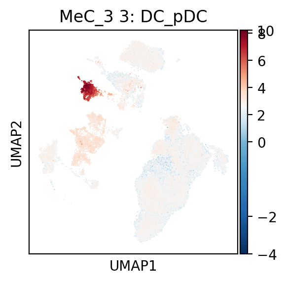
Plot signature continuum for a single MeC

[14]:

fig=plmapper.plot_umap_mec( pdata, 'MeC_3' ,mecnamedict, figfile =None)

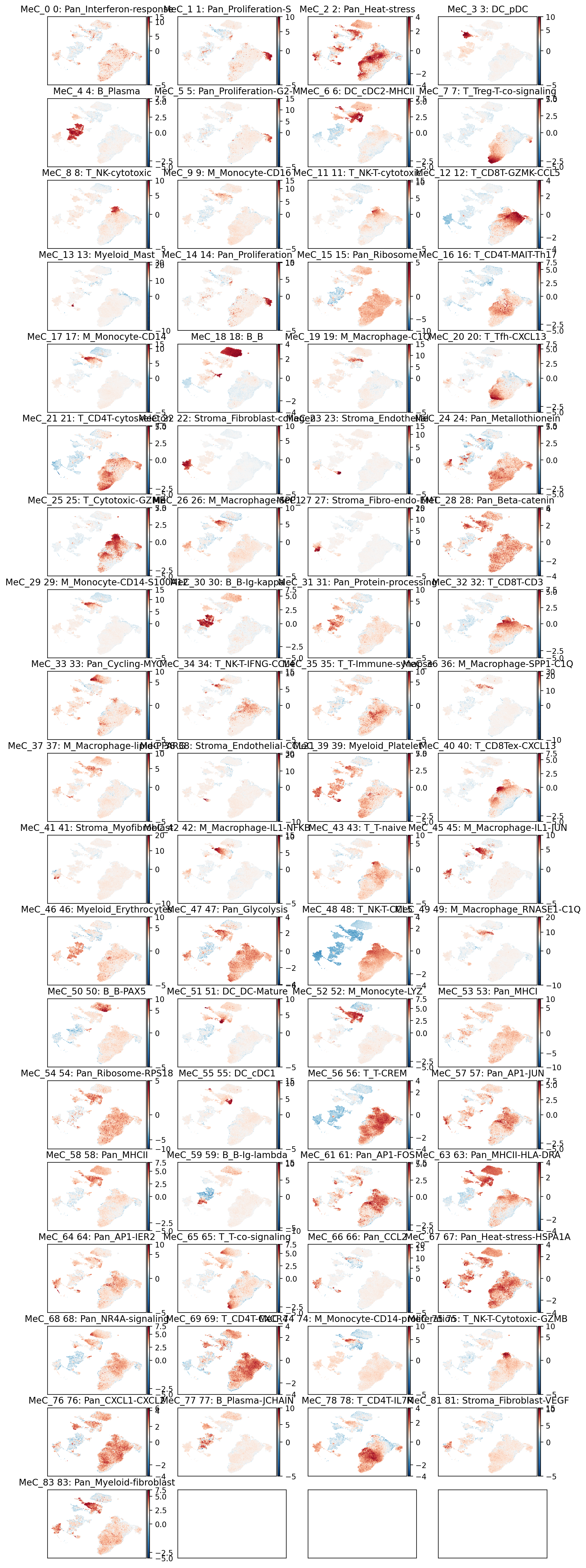
../_images/notebooks_metatime_annotator_42_0.png

Plot signature continuum for all functional MeCs

[15]:

fig=plmapper.plot_umap_proj_pdata( pdata, mecnamedict , figfile =None)

../_images/notebooks_metatime_annotator_44_0.png

Comparing conditions

The first way is to count cells newly annotated by MetaTiME. A count table can be returned in all ways grouping the cells. The conditions here are dataset - specific.

[16]:

condcol = 'treatment'
clustercol = 'MetaTiME'
samplecol = 'patient'

cellcts = dmec.count_cell_condition( adata.obs, countbycols = [condcol, clustercol, samplecol] )
#cellcts.to_csv('./cell_counts.txt',sep='\t')
cellcts

[16]:

	patient	su001	su002	su003	su004	su005	su006	su007	su008	su009	su010	su012
treatment	MetaTiME
post	B_B	3447.0	0.0	8.0	19.0	55.0	18.0	2.0	127.0	2.0	0.0	0.0
	B_B-Ig-kappa	12.0	3.0	0.0	3.0	8.0	537.0	0.0	27.0	0.0	0.0	2.0
	B_B-Ig-lambda	7.0	1.0	1.0	2.0	3.0	76.0	2.0	32.0	0.0	0.0	0.0
	B_B-PAX5	273.0	0.0	0.0	0.0	0.0	0.0	0.0	0.0	0.0	0.0	0.0
	B_Plasma	15.0	4.0	0.0	5.0	16.0	164.0	2.0	23.0	8.0	0.0	2.0
...	...	...	...	...	...	...	...	...	...	...	...	...
pre	T_T-CREM	72.0	4.0	7.0	33.0	64.0	83.0	126.0	12.0	324.0	7.0	100.0
	T_T-Immune-synapse	47.0	0.0	6.0	22.0	28.0	35.0	82.0	4.0	146.0	6.0	130.0
	T_T-naive	1.0	0.0	2.0	13.0	13.0	2.0	22.0	1.0	113.0	0.0	13.0
	T_Tfh-CXCL13	25.0	2.0	9.0	16.0	74.0	335.0	94.0	87.0	408.0	0.0	465.0
	T_Treg-T-co-signaling	200.0	6.0	8.0	52.0	79.0	300.0	166.0	90.0	338.0	3.0	353.0

76 rows × 11 columns

Writing the cell counts to table

[22]:

cellcts.to_csv('./cell_counts.txt',sep='\t')

MetaTiME also provides functions to test differential signatures cluster-wise.

[17]:

condcol = 'treatment' # the column in adata.obs to mark the condition
cond1 = ['pre'] # Condition 1 in adata.obs[ condcol ],
cond2 = ['post'] # Condition 2 in adata.obs[ condcol ],
clustercol = 'MetaTiME' # MetaTiME annotated cluster labels


# get the cell barcodes for two conditions
allcellscond1= adata[adata.obs[ condcol ].isin(cond1), ].obs.index
allcellscond2= adata[adata.obs[ condcol ].isin(cond2), ].obs.index

[18]:

print(f'Compare cells based on {condcol} with conditions {cond1} and {cond2}')
print(f'Cells in Condition {cond1} : {len(allcellscond1)}')
print(f'Cells in Condition {cond2} : {len(allcellscond2)}')

Compare cells based on treatment with conditions ['pre'] and ['post']
Cells in Condition ['pre'] : 13710
Cells in Condition ['post'] : 25126

Get A table listing all signatures enriching in each cluster, as candidate for testing differential signature.

[19]:

mec_enriched = dmec.enrich_mec(
    adata=pdata, labelcol =clustercol, mecnamedict=mecnamedict_simp)

Testing all candidate signatures in each cell cluster.

[20]:

diffmec, diffmecsig, diffmec_full = dmec.dmec(adata, pdata, allcellscond1, allcellscond2, clustercol, mec_enriched, mecnamedict_simp,
                                              test_clusters='all', test_method = 'ttest' )

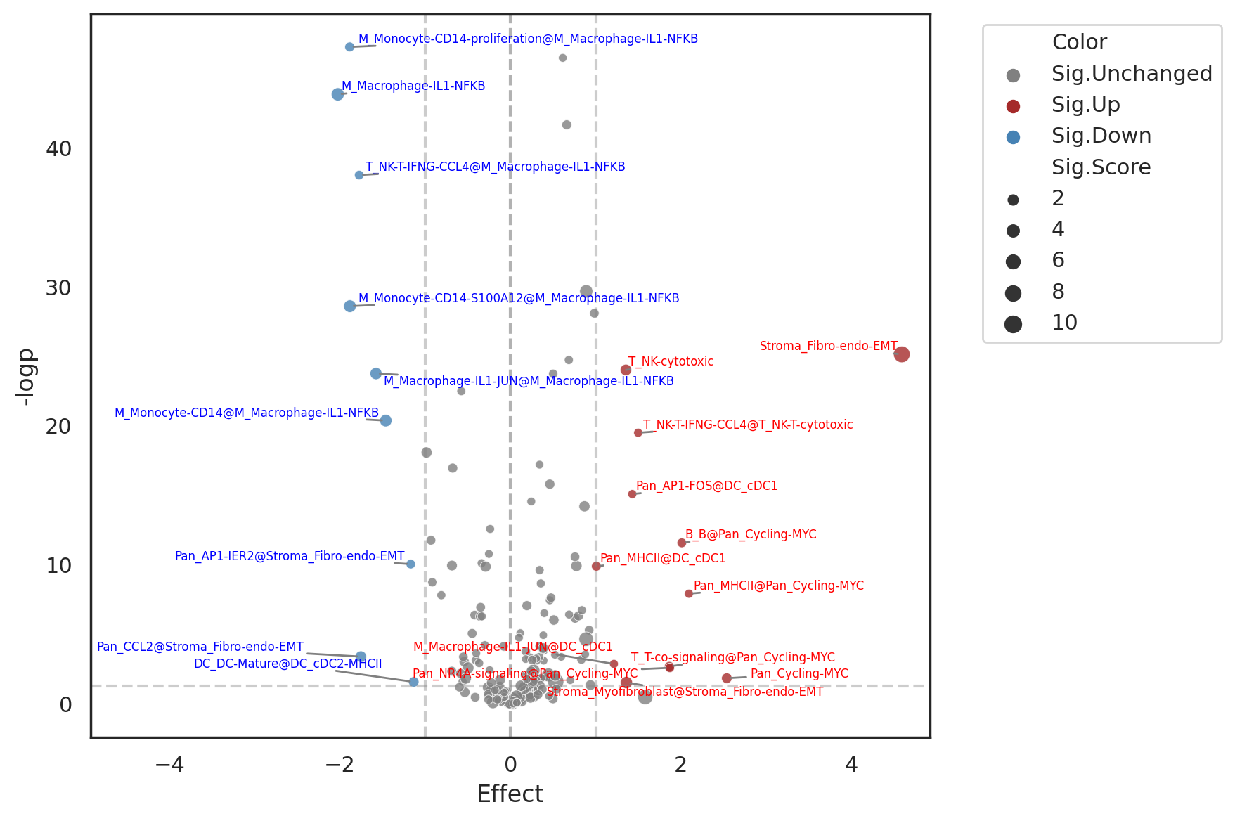
Plotting the differential signature dot plot.

X-axis: difference of mean signature scores between conditions. Y-axis: -⁡log(p-value) from the test statistic chosen. The significant cluster-wise differential signature is marked as “EnrichedMeC@ClusterName”; when the enriched MeC is the same as cluster name, the signature is marked “ClusterName”. Size of the dots is proportionally to the mean signature score.

[27]:

sns.set_theme(style='white')
fig_topdiff = dmec.plot_topdiff(diffmec, fontsize=6)

../_images/notebooks_metatime_annotator_60_0.png

Save all the significant differential signatures@Cluster

[24]:

diff, diff_sig = dmec.topdiff_df(diffmec)

[25]:

diff_sig[:3]

[25]:

	-logp	effect	effect1	meanb	meana	scorecol	cluster1	mec
M_Monocyte-CD14-proliferation@M_Macrophage-IL1-NFKB	47.236925	-1.885173	-1.885173	0.486959	2.372133	MeC_74	M_Macrophage-IL1-NFKB	M_Monocyte-CD14-proliferation
M_Macrophage-IL1-NFKB	43.831255	-2.024648	-2.024648	4.083235	6.107882	MeC_42	M_Macrophage-IL1-NFKB	M_Macrophage-IL1-NFKB
T_NK-T-IFNG-CCL4@M_Macrophage-IL1-NFKB	38.030503	-1.774028	-1.774028	0.264443	2.038471	MeC_34	M_Macrophage-IL1-NFKB	T_NK-T-IFNG-CCL4

Saving this table

[36]:

diff_sig.to_csv('diff_sig_allcluster.txt',sep='\t')